It works by iterating the input array from the first element to the last, comparing each pair of elements and swapping them if needed.
Complexity : n2
Algorithm -> A[] and size
pass , i;
for ( pass = size-1 ; pass > 0; pass--)
for (i = 0; i<pass ; i++)
if(A[i] > A[i+1])
Swap A[i] and A[i+1] with the help of temp variable
Algorithm takes O( n2) (even in best case). We can improve it by using one extra flag. See below program for implementation with flag = swapped BubbleSort Program
Best Case complexity of improved version is O(n)
Advantage
It can detect whether the input array/list is already sorted or not
Selection Sort
This algorithm is called selection sort since it repeatedly selects the smallest element. Selection sort is an in-place sorting algorithm. It comes under greedy algorithm because at each step it tries to find the min, though being greedy does not mean that it will result in optimal solution See Program
Complexity : n2
Algorithm -> A[] and size
int i , j , min , temp
for( i = 0 ; i <= size-1 ; i++)
min = i
for( j = i+1 ; j < size ; j++)
if A[j] < A[min]
min = j
swap A[i] and A[min] using temp
Advantage
In place sorting
Insertion Sort
Advantage
In-place: It requires only a constant amount O( 1) of additional memory space
Online: Insertion sort can sort the list as it receives it
Merge Sort:
Merging is the process of combining two sorted files to make one bigger sorted file.
In Quick sort most of the work is done before the recursive calls. Quick sort starts with the largest subfile and finishes with the small ones and as a result it needs stack. Moreover, this algorithm is not stable. Merge sort divides the list into two parts; then each part is conquered individually. Merge sort starts with the small subfiles and finishes with the largest one. As a result it doesn’t need stack. This algorithm is stable.
Difference between Dynamic Programming and Divide and Conquer
The main difference between dynamic programming and divide and conquer is that in the case of the latter, sub problems are independent, whereas in DP there can be an overlap of sub problems.
By uing memoization [maintaining a table of sub problems already solved], dynamic programming reduces the exponential complexity to polynomial complexity (O( n2), O( n3), etc.) for many problems.
The major components of DP are:
Recursion: Solves sub problems recursively.
Memoization: Stores already computed values in table (Memoization means caching).
Dynamic Programming = Recursion + Memoization
Problems:
Books Problem
Problem1: Convert the following recurrence to code.
The D & C algorithm works by recursively breaking down a problem into two or more sub problems of the same type, until they become simple enough to be solved directly. The solutions to the sub problems are then combined to give a solution to the original problem.
The D & C strategy solves a problem by:
Divide: Breaking the problem into sub problems that are themselves smaller instances of the same type of problem.
Recursion: Recursively solving these sub problems.
Conquer: Appropriately combining their answers.
Does D&C always work?
As per the definition of D & C, the recursion solves the subproblems which are of the same type. For all problems it is not possible to find the subproblems which are the same size and D & C is not a choice for all problems.
As an example, consider the Tower of Hanoi problem. This requires breaking the problem into subproblems, solving the trivial cases and combining the subproblems to solve the original problem. Dividing the problem into subproblems so that subproblems can be combined again is a major difficulty in designing a new algorithm. For many such problems D & C provides a simple solution.
Advantages of D&C:
Solving Difficult Problems
Parallelism : Since sub problems can be solved independently, multiprocessor machines like shared memory system need not be planned in advance.
Memory Access : D & C algorithms naturally tend to make efficient use of memory caches. This is because once a subproblem is small, all its subproblems can be solved within the cache, without accessing the slower main memory.
Disadvantages of D&C:
Recursion is slow i.e. Since it needs stack for storing the calls but the overhead of recursion is negligible with large enough recursive base cases.
It can be more complicated than iterative approach if the problem is simple.
Huffman coding algo is used to compress data using greedy choice so that it does not loose any information.
Example: A is given value 000, Frequency is 10, now since 000 is 3 bits, Total bits is 3x10 = 30
For E -> 3x15 = 45(total bits)
Total bits = 174
We can represent the above example in tree form as:
Our AIM:
To reduce the traversal through the code tree to the nodes which has the highest frequency
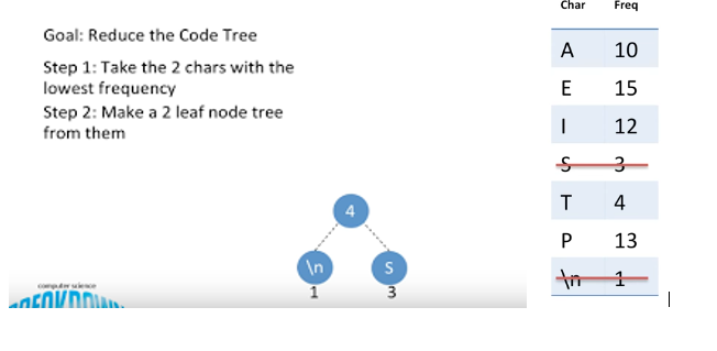
Step3: Add the next 2 nodes and add their frequency and add to the tree. Goes on
We keep on adding the nodes frequency and making tree, but 18 is more than the highest frequency i,e,15, hence we can no longer keep on adding nodes to this tree.
Hence we add next two lowest frequency to another subtree. Now since only E is left, we will add it to the tree which has lowest root value.
Example: Game of chess - when we play a move, we have to also think about the future consequences. Whereas, in the game of Tennis (or Volleyball), our action is based on the immediate situation.
The Greedy technique is best suited for looking at the immediate situation.
Greedy Strategy
Greedy algorithms work in stages. In each stage, a decision is made that is good at that point, without bothering about the future. This means that some local best is chosen. It assumes that a local good selection makes for a global optimal solution.
Two basic properties of optimal Greedy algorithms
Greedy choice property
This property says that the globally optimal solution can be obtained by making a locally optimal solution
Optimal substructure
A problem exhibits optimal substructure if an optimal solution to the problem contains optimal solutions to the subproblems. That means we can solve subproblems and build up the solutions to solve larger problems.
Note: Making locally optimal choices does not always work.
Advantage:
We do not have to spend time re-examining the already computed values, once decision is made.
Disadvantage:
In many cases there is no guarantee that making locally optimal improvements in a locally optimal solution gives the optimal global solution.
In computer science each field has its own problems and needs efficient algorithms. Examples: search algorithms, parallel algorithms, data compression algorithms, parsing techniques, and more.
Classification by Complexity
In this classification, algorithms are classified by the time they take to find a solution based on their input size. Some algorithms take linear time complexity (O( n)) and others take exponential time, and some never halt.
Classification by Complexity
In this classification, algorithms are classified by the time they take to find a solution based on their input size. Some algorithms take linear time complexity (O( n)) and others take exponential time, and some never halt.
Branch and Bound Enumeration and Backtracking
These were used in Artificial Intelligence and we do not need to explore these fully. For the Backtracking method refer to the Recursion and Backtracking chapter.